Metrics

Machine learning metrics are quantitative measures used to evaluate the performance of a machine learning model, and a confusion matrix is a specific type of metric that provides a comprehensive summary of the model's predictions by comparing them to the actual class labels.

Goals

By the end of this lesson, you should be able to:

• Calculate confusion matrix, precision, and recall.

Keywords

metrics, confusion matrix, accuracy, precision, sensitivity, specificity, positive case, negative case

Introduction

In Linear Regression, we use the correlation coefficient and some mean square errors as metrics to see if our model fits the data well. What kind of metrics we can use in the case of classification problems? In this lesson we will use confusion matrix and a few matrix to evaluate our classification model.

Confusion Matrix

Recall in the first lesson on machine learning, we give an example of classifying image as cat or not a cat. Now, let's say we have a dataset of images of various animals including some cats picture inside. First, we need to separate the dataset into training set and test set. The training set is used to build the model or to train the model. Our model for classification which we discussed in the previous lessson was called Logistic Regression. After we train the model, we would like to measure how good the model is using the test set. We can write a table with the result of how many data is predicted correctly and not correctly as shown below.

actual\predicted	a cat	not a cat
a cat	11	3
not a cat	2	9

The above table gives some example of what is called as a confusion matrix. The vertical rows are the labels for the actual data while the horizontal columns are the labels for the predicted data. We can read this table as follows.

• Out of all the actual image which is a cat, 11 images are predicted as a cat and 3 images are predicted as not a cat. This means that 11 of them are accurate and 3 of them is not.
• Out of all the actual image which is not a cat, 2 images are predicted as a cat and 9 images are predicted as not a cat. This means that 2 of them are not accurate and 8 is.

We can see that there are a total of $11+3=14$ images of the category a cat. On the other hand, there are $2+9=11$ images of the category a cat. So the total number of images are $11 + 3 + 2 + 9 = 25$ images.

The confusion matrix in general is written as follows.

actual\predicted	Positive Case	Negative Case
Positive Case	True Positives	False Negatives
Negative Case	False Positives	True Negatives

We use the term positive case here to refer to the category of point of interest. In this case, we would like to detect a cat and so category a cat is a positive case. On the other hand, the category not a cat is a negative case. This means that:

• There are 11 True Positive cases where the actual cat images are predicted as a cat.
• There are 9 True Negative cases where the actual not a cat images are predicted as not a cat.
• There are 3 False Negative cases where the actual cat images are predicted as not a cat (negative case).
• There are 2 False Positive cases where the actual not. acat images are predicated as a cat (positive case).

Metrics

Knowing the confusion matrix allows us to compute several other metrics that is useful for us to evaluate our model.

Accuracy

In this metrics, we are interested in how many data is predicted correctly. In the above examples, we have 11 images predicted correctly as cats and 9 images predicted correctly as not a cat. Therefore, we have the accuracy of:

$$\text{accuracy} = \frac{11 + 9}{25} = \frac{20}{25} = 0.8$$

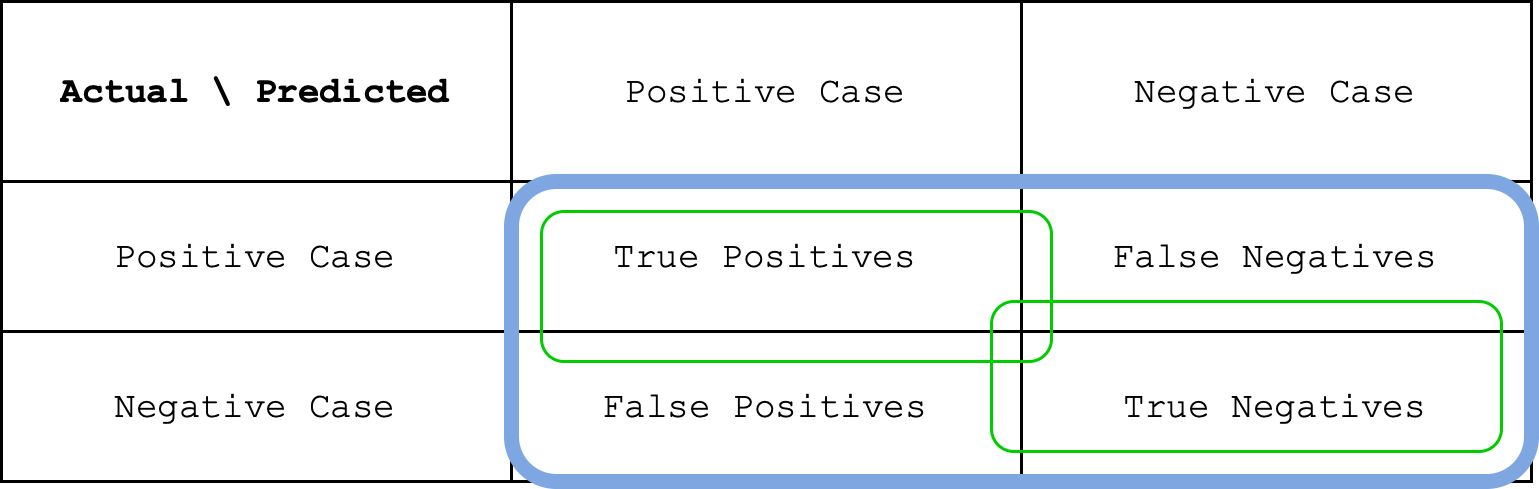
This means our model have 80% accuracy. In general, the accuracy formula can be written as:

$$\text{accuracy} = \frac{\text{TP} + \text{TN}}{\text{Total Cases}}$$

where TP is the number of True Positive cases, TN is the number of True Negative cases. You can also see accuracy as a fraction of the green circle over the blue circle in the image below.

Given the accuracy, we can also calculate another metric called error rate. In fact, the error rate is just given by the following:

$$\text{error rate} = 1 - \text{accuracy}$$

So in our example, the error rate is $1 - 0.8 = 0.2$ which is 20%.

Precision

In precision, we put more attention into the positive cases. We are interested in how many of the positive cases are detected accurately.

actual\predicted	a cat	not a cat
a cat	11	3
not a cat	2	9

$$\text{precision} = \frac{11}{11 + 2} = \frac{11}{13} = 0.846$$

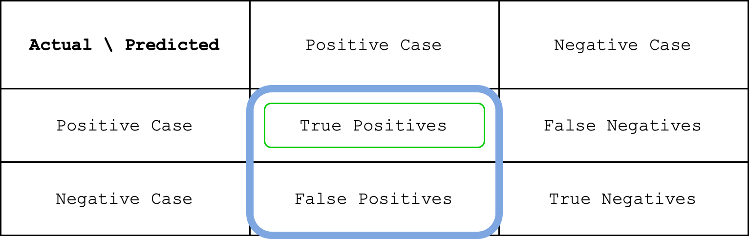
This means that we have a precision of about 85\%. Out of all the total 13 cases detected positive, 11 of them is correct. Obviously we want our precision to be as high as possible. We can write precision formula as follows.

$$\text{precision} = \frac{\text{TP}}{\text{Total Predicted Positives}} = \frac{\text{TP}}{\text{TP} + \text{FP}}$$

The calculation of precision can be seen as a fraction between the green circle and the blue circle in the image below.

Sensitivity

This is also often called as Recall. In this metric, we are interested to know the fraction of the number of positive cases predicted accurately out of all the actual positive cases. The difference with precision is that precision is calcalculated as a fraction out of all the total predicted positive cases. In the above example, we have 11 true positives and the total number of all actual positive cases are $11 + 3 = 14$.

actual\predicted	a cat	not a cat
a cat	11	3
not a cat	2	9

$$\text{sensitivity} = \frac{11}{11 + 3} = \frac{11}{14} = 0.786$$

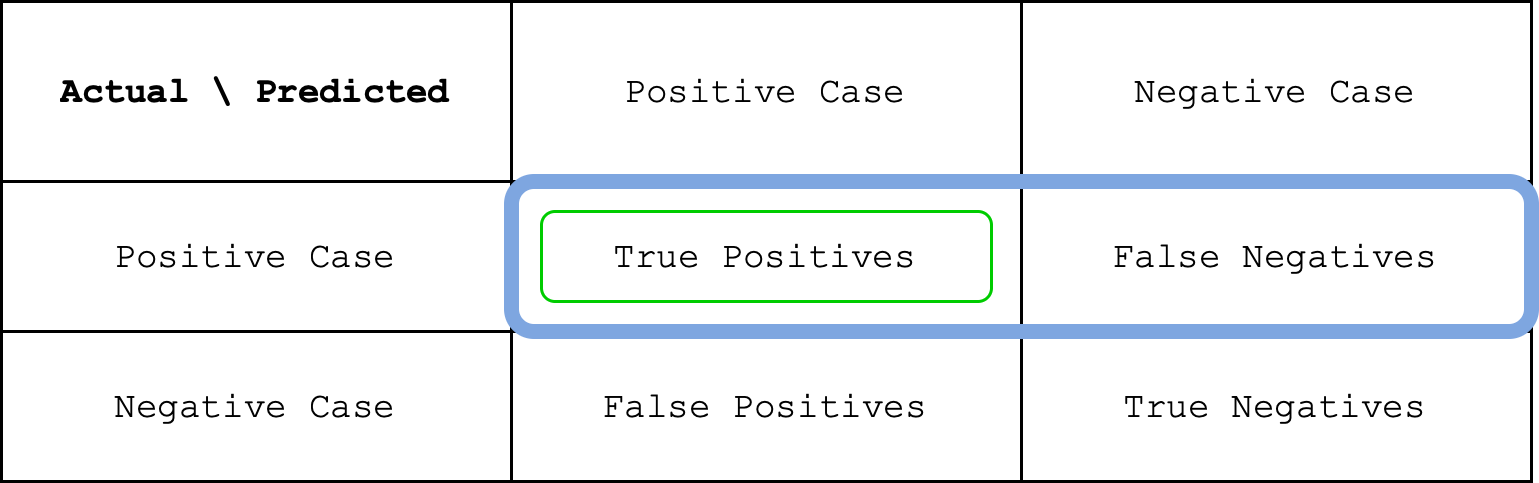
This means that the sensitivity is about 79\%. Notice that the sensitivy value is different from precision which is about 85\%. We can write the formula for sensitivity as follows.

$$\text{sensitivity} = \frac{\text{TP}}{\text{Total Actual Positives}} = \frac{\text{TP}}{\text{TP} + \text{FN}}$$

We can see sensitivty as a fraction between the green circle and the blue circle in the image below.

Specificity

Another common matrix is called specificity. This is the metrix we normally use when we are interested in the negative cases. It is also called as True Negative Rate. Specificity is calculated as the number of True Negative cases divided over all actual Negative cases.

actual\predicted	a cat	not a cat
a cat	11	3
not a cat	2	9

$$\text{specificity} = \frac{9}{9 + 2} = \frac{9}{11} = 0.818$$

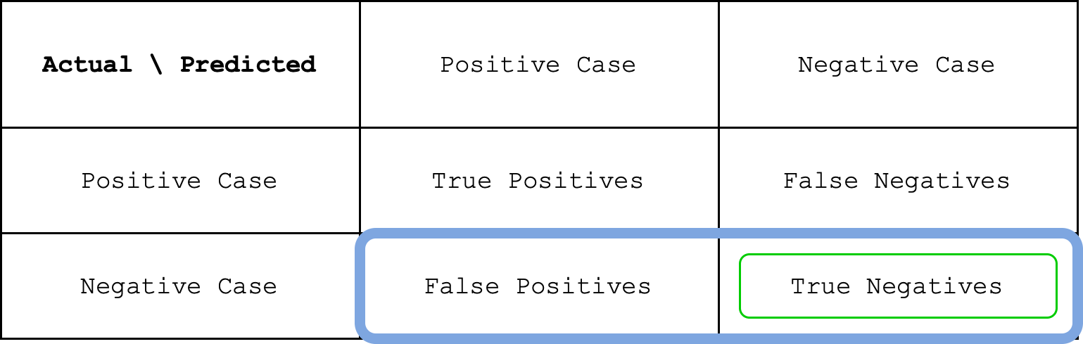
This means that the true negative rate is about 82\%. You can see specificity as the sibling of sensitivity. In sensitivity, you are interested in the positive cases while in the specificity you are interested in the negative cases. The formula for specificity is given as follows.

$$\text{specificity} = \frac{\text{TN}}{\text{Total Actual Negatives}} = \frac{\text{TN}}{\text{FP} + \text{TN}}$$

We can see specificity as a fraction between the green circle and the blue circle in the image below.

Confusion Matrix for Multiple Classes

What if we have more than two categories. What would the confusion matrix look like? Let's say we are classifying images of cat, dog, and a fish. In this case, we have three categories. We can write our confusion matrix in this manner.

actual\predicted	cat	dog	fish
cat	11	1	2
dog	2	9	3
fish	1	1	8

The diagonal element again gives us the accuracy of the model.

$$\text{accuracy} = \frac{11 + 9 + 8}{38} = \frac{28}{38} = 0.737$$

which is about 73\%. We can write the formula for accuracy as follows.

$$\text{accuracy} = \frac{\sum_i M_{ii}}{\sum_i\sum_j{M_{ij}}}$$

The formula simply sums up all the diagonal elements and divide it with the sum of all.

We can calculate the other metrices by defining our positive case in a one-versus-all manner. This means that if we define cat as our positive case, we define both dog and fish as the negative cases.

For example, to calculate the sensitivity for class i, we use:

$$\text{sensitivity}_i = \frac{M_{ii}}{\sum_j{M_{ij}}}$$

where $i$ is the class we are interested. The summation over $j$ means we sum over all the columns in the confusion matrix.

Similarly, we can calculate the precision for class i using:

$$\text{precision}_i = \frac{M_{ii}}{\sum_j{M_{ji}}}$$

Notice that the indices are swapped for the denominator. For precision, instead of summing over all the columns, we sum over all the rows in column i which is the total cases when class i is predicted.