Merge Sort

Merge Sort is another sorting algorithm that implements the principle of divide and conquer.

Goals

By the end of this lesson, you should be able to:

Explain and implement merge sort algorithm
Derive solution of recurrence of merge sort using recursion-tree method
Measure computation time of merge sort and compare it with the other sort algorithms

Keywords

sorting, mergesort, log linear time complexity

Introduction

The previous example of summing an array gives a simple example of divide-and-conquer approach as an alternative to iterative solution. We also showed another problem which is easier to solve recursively as in the problem of Tower of Hanoi. Now, we will give another example which is intuitively recursive, merge sort algorithm.

Merge sort follows the three steps divide, conquer, and combine. The idea of merge sort is split the input sequence into two parts (divide), and call merge sort recursively on each parts (conquer). After the two parts are sorted, it is then combined using merge step (combine).

Algorithm

(P)roblem Statement

The problem statement is the same as any other sorting problem. Given an arbitrary sequence of numbers, say Integers, the problem is sequence this number in a certain order, say from smallest to largest.

Test (C)ase

Let's give an example for a particular input sequence and see how merge sort solves the problem.

[16, 14, 10, 8, 7, 8, 3, 2, 4, 1]

We split the array into two parts recursively until each array is left only with one element.

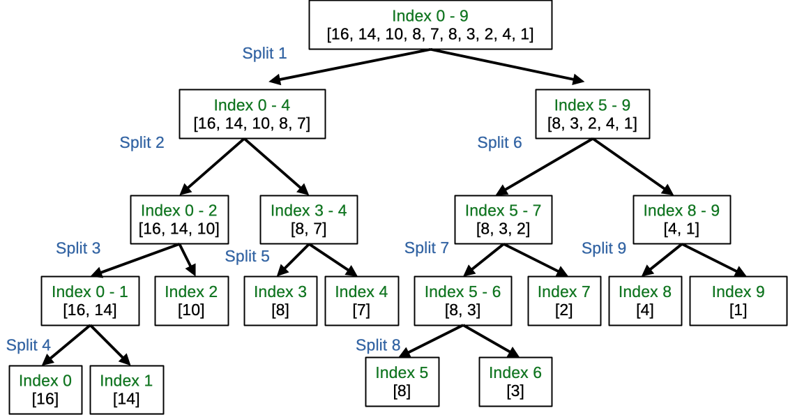
When we have the array with only one element, the array is trivially sorted. So now what we can do is to go up and merge the two array. This is shown in the figure below.

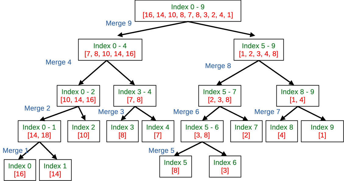
How do we merge the two arrays? We will give this example in the merge of the last step to get the final sorted array.

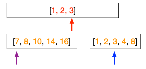
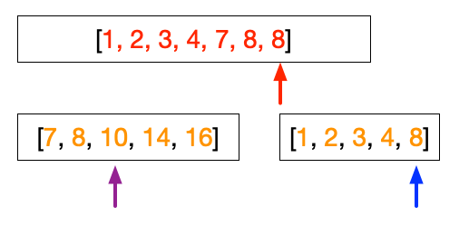
The merge steps have three arrows as shown in the figure below, the red, purple, and blue. The red arrow points to the position of where to store the number in the sorted array. The purple arrow points to the number in the left array while the blue arrow points to the number in the right array. The merge step begins by comparing the number pointed by the purple arrow with the number pointed by the blue arrow. We then put the smaller number into the sorted array.

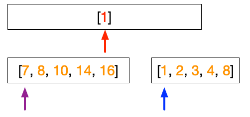
We then move the arrow from which we move the number. In the example above 1 is smaller than 7, therefore, we put 1 into the position pointed by the red arrow and move the blue arrow to the next number.

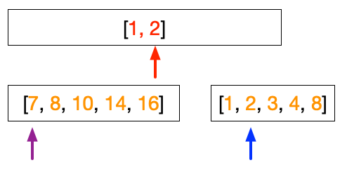
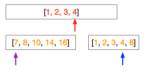
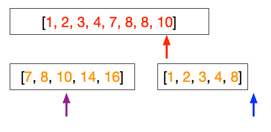
These steps continue as follows.

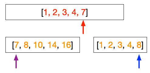
At this point, both left and right array have the same value, i.e. 8. We can choose arbitrarily that when the value is the same, we will take the value from the left array.

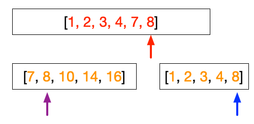
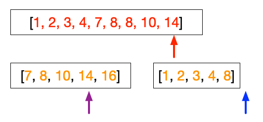
At this point, we have finished putting the right array. So the subsequent steps simply filling up the sorted array from the left array.

(D)esign of Algorithm

As shown in the previous section, we can divide Merge sort into two algorithm. The first algorithm is the main steps that contains the recursive calls. The second algorithm is the merge steps. We will discuss both algorithms below.

In designing the main steps, we identify the recursive case and the base case. In our case, the base case is when the array contains only one element. In this case, the array is trivially sorted. Therefore, we do not need to do anything. On the other hand, when the number of element in the array is greater than one, we split the array into two, and call recursively the same steps, and combine them after they are sorted. We can write the algorithm in this way.

Show Pseudocode

Merge Sort
Input:
 - array = sequence of integers
 - p = index of beginning of array
 - r = index of end of array
Output: None, sort the array in place
Steps:
1. if r - p > 0, do:
    1.1 calculate q = (p + r) / 2
    1.2 call MergeSort(array, p, q)
    1.3 call MergeSort(array, q+1, r)
    1.4 call Merge(array, p, q, r)

Note:

We only consider the recursive case in step 1, i.e. when the length of the array we consider is more than one items. The base case is trivial since it is sorted if there is only one element. We know it is only one element if the end index and the beginning index is greater than 0.
Then we calculate the middle point to split the array, i.e. $q = (p+r)/2$ .
We can then call the procedure recursively. Step 1.2 is to sort the left array which is from index $p$ to index $q$ while step 1.3 is to sort the right array which is from index $q+1$ to index $r$ .
Step 1.4 is the combine step by calling the merge procedure.

We can now discuss the merge step algorithm. To do this step, we have three indices, we will call them left (purple), right (blue), and dest (red). The idea is to start from the beginning and compare the numbers pointed by the left and the right arrow. The smaller number will placed in position pointed by dest.

Show Pseudocode

Merge
Input:

- array = sequence of integers
- p = beginning index of left array, which is also the beginning of the input sequence
- q = ending index of left array
- r = ending index of right array
  Output: None, sort the array in place
  Steps:

nleft = q - p +1
nright = r - q
left_array = array[p...q]
right_array = array[(q+1)...r]
left = 0
right = 0
dest = p
As long as (left < nleft) AND (right < nright), do:
1 if left_array[left] <= right_array[right], do:
1.1 array[dest] = left_array[left]
1.2 left = left + 1
2 otherwise, do:
2.1 array[dest] = right_array[right]
2.2 right = right + 1
3 dest = dest + 1
As long as (left < nleft), do:
1 array[dest] = left_array[left]
2 left = left + 1
3 dest = dest + 1
As long as (right < nright), do:
1 array[dest] = right_array[right]
2 right = right + 1
3 dest = dest + 1

Note:

Steps 1 and 2 are used to calculate the numbe of elements in the left and right arrays.
Steps 3 and 4 are to copy the elements from the input array to the left and the right arrays.
Step 5 and 6 are to initialize the position of the left and right array. We use index 0 here because we copied the numbers into two new arrays. The new arrays start with index 0.
Step 7 is to initialize the dest arrow. It starts from p which is the starting of the sorted array.
Step 8 is the merging steps by comparing the two arrays.
Step 8.1 is the comparison to choose which element should be put into the sorted array. If the number in the left array is smaller than that number is placed into the sorted array (Step 8.1.1) and the arrow moves to the next number (Step 8.1.2). Otherwise, it will place the number from the right array (Step 8.2).
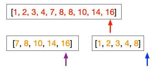
Step 9 and 10 is to handle when the left array and the right array do not have the same length. In this case, the iteration in step 8 will terminate once the arrow reaches the end of the shorter array. In the figures above, we finish the right array before the left array. The last three figures above are simply the steps taken by Step 9 in putting the numbers 10, 14, and 16 into the sorted array.

Computation Time

We will use the recursive tree method to analyze the computation time taken by Merge Sort. Looking into the pseudocode of Merge Sort, we can write the computation time as

T_{mergesort}(n) = O(1) + 2T_{mergesort}(n/2)+T_{merge}(n)

Note:

the constant time $O(1)$ comes from the comparison and the calculation of the index $q$ . These takes constant time.
there are two recursive call of merge sort for the left and the right right. This results in $2T_{mergesort}(n/2)$ .
there is a call to merge procedure which gives $T_{merge}(n)$ .

Therefore, in order to find the computation time for the merge sort, we need to look into the computation time for the merge procedure. Looking into the pseudocode of Merge, we can note the following:

Steps 1 and 2 are constant time. Similarly for steps 5 to 7. This contributes to $O(1)$ .
The copying to left and right array depends on the number of elements and so $O(n)$ .
Steps 8, 9 and 10 are taken to insert the numbers into the sorted array. These are done in total of $n$ times because the final result is $n$ elements in the sorted array. This means that it is also $O(n)$ .
The sub steps inside 8, 9 and 10 are all constant times which is repeated for $n$ times.

Therefore, the merge step computation time can be written as:

T_{merge}(n) = O(1) + O(n) + O(n)\times(O(1)) = O(n)

Combining all the timing, we then have the following for the merge sort computation.

T(n) = \begin{cases}O(1), & \text{if } n=1\\ 2T(n/2) + O(n), & \text{if } n > 1\end{cases}

So now for $n>1$ , we have the recurrence relation as follows:

T(n) = 2 T(n/2) + c n

where $c$ is a constant and $c > 0$ .

We can draw the recurrence tree as shown in the figure below.

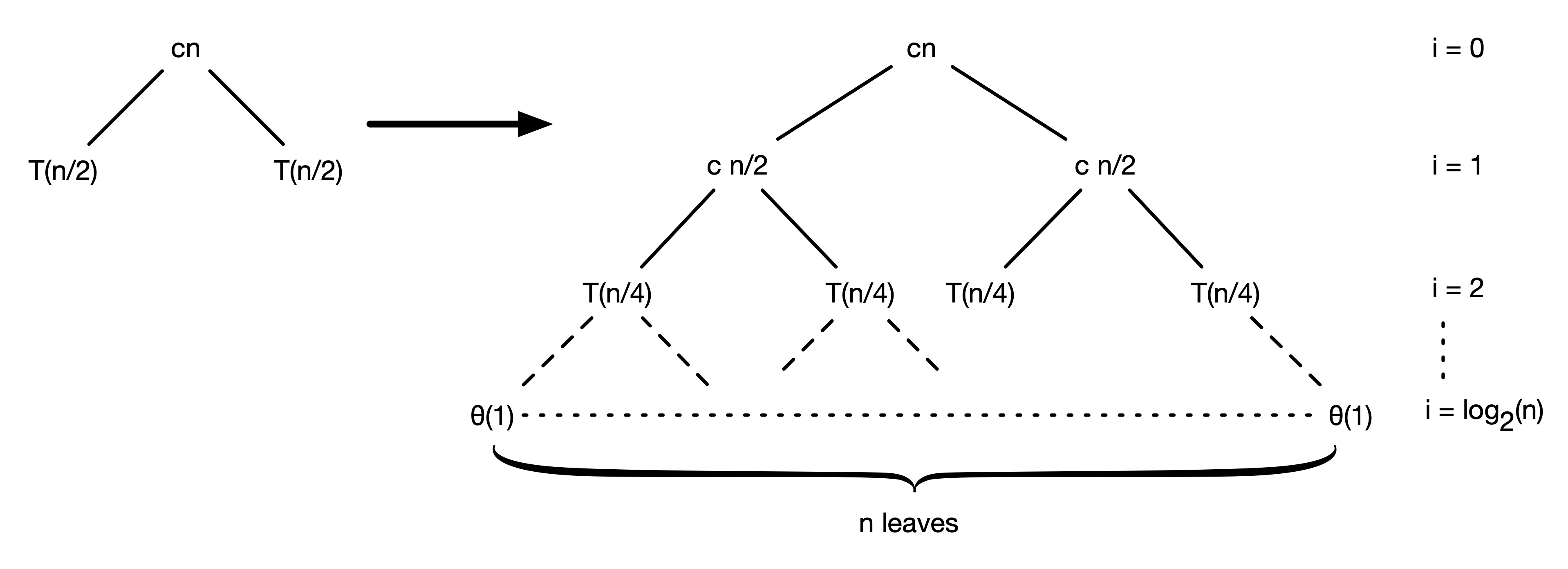
Note that at the bottom of the tree, there are $n$ leaves, where $n$ is the number of input in the array. We can also calculate the level at the bottom. At every level, the computation time at each node in the recurrence tree is given by:

\frac{cn}{2^i}

For example, at $i = 1$ , the computation time is

\frac{cn}{2^1} = \frac{cn}{2}

At the bottom of the tree, we can only $c\times 1$ . Therefore, we have the following relationship.

\frac{cn}{2^{i_{bottom}}} = c \times 1

and we can get

i_{bottom} = \log_2(n)

This means that the height of the tree is:

h = 1 + \log_2(n)

And if we sum up the computation time at each leve, we would obtain $c\times n$ . For example at level $i = 1$ , we have

cn/2 + cn/2 = cn

and similarly at every level. Therefore, the total computation time is the sum at each level multiplied by the number of level.

T(n) = cn \times (1 + \log_2(n)) = O(n\log(n))

Here and the subsequent expressions, we always use base of 2 for our logarithmic function.

Note that the computation time is slower than linear but much faster than quadratic time. This means that merge sort gives a faster computation time as compared to bubble sort and insertion sort and is similar to heapsort.

Merge Sort

Goals​

Introduction​

Algorithm​

(P)roblem Statement​

Test (C)ase​

(D)esign of Algorithm​

Computation Time​

Goals

Introduction

Algorithm

(P)roblem Statement

Test (C)ase

(D)esign of Algorithm

Computation Time