Breadth First Search

Breadth-first search is a graph traversal algorithm that explores all the vertices of a graph at the same level before moving to the next level, ensuring the shortest path to each vertex is discovered first.

Goals

By the end of this lesson, you should be able to:

• explain and implement breadth first search

Keywords

graph traversal, breadth first search, distance, colour, parent vertex, inheritance, child class, parent class, super

Introduction

In the previous lesson, we have introduced how we can represent a graph using object oriented programming. We created two classes Vertex and Graph. One main use cases with this kind of data is to do some search. For example, given the graph of MRT lines, we would like to search what is the path to take from one station to another station. We usually are interested in the shortest path. This is what Google Map and other Map application does. In this lesson, we will discuss two graph search algorithms: breadth-first search and depth-first search.

To do these algorithms, our Vertex class and Graph class may need some additional attributes to store more information as it performs the search. One way to modify our classes is to create a new class. However, we would like to introduce the concept of Inheritance. Inheritance allows us to re-use our existing class and create a new class that is derived from our existing class. Therefore, to implement our search algorithm, we will use inheritance to modify our existing Vertex and Graph classes.

Breadth First Search

Breadth first search is normally used to find a shortest path between two vertices. For example, when you plan your travel from one point to another point, breadth first search can identify the path you should take that gives the shortest path. How does this work? Let's take a look at the graph below.

(C)ases

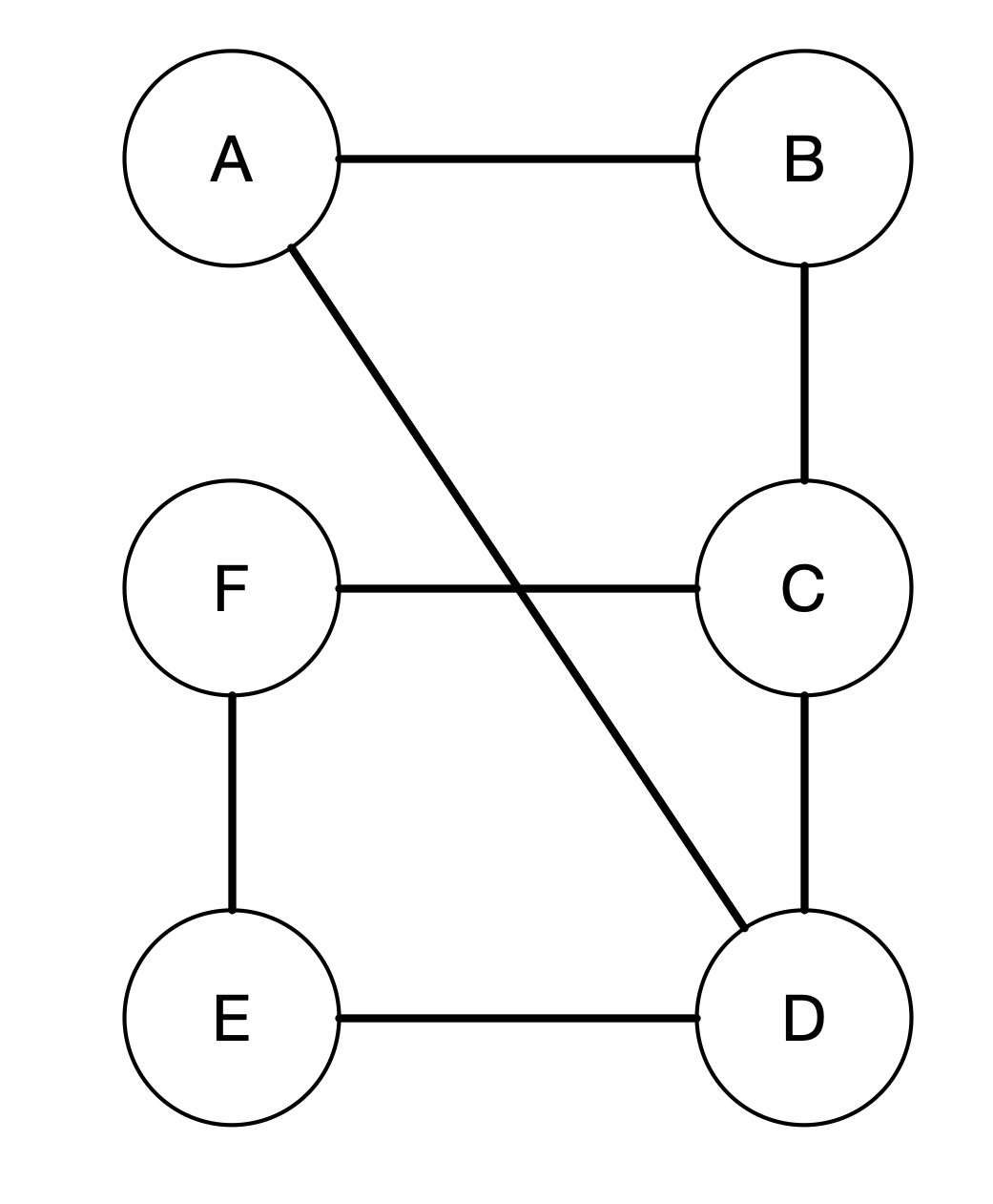
Let's say we want to find the shortest path from A to F. The way breadth-first search does is to calculate the distance of every vertex from A. So in this case, B will have a distance of 1 since it takes only one step from A to B. On the other hand, C has a distance of 2. D, however, has a distance of 1 since there is an edge from A to D connecting the two vertices directly. Vertex E has a distance 2 because from A it can go to D and then to E in two steps. Finally, F has a distance of 3. There are actually two paths from A to F. The first one is A - B - C - F and the second one is A - D - E - F. Notice that both has the same distance, which is 3.

How can we obtain all the distances for each vertex? We will start with the starting vertex which in this case is A. Next, we can look into the neighbouring vertices that A has. So in this case, A has two neighbours, i.e. B and D. We can then explore each of the neighbours. We can draw the the vertex that we are exploring as a kind of a tree.

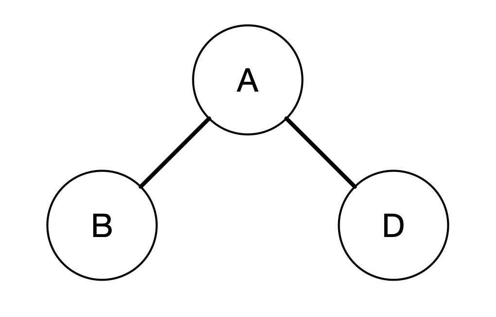
We can then take turn to explore the neighbours of each of the children in the tree. In this case, B has two neighbours, i.e. A and C. But since we have visited A, we do not want to visit A again. So we should only visit C. This indicates that we need to mark the vertices that we have visited. Similarly, D has three children, i.e. A, C and E. But both A and C has been visited, so we should just add E into our tree. We can continue the same steps until all vertices have been visited. The final tree looks like the following.

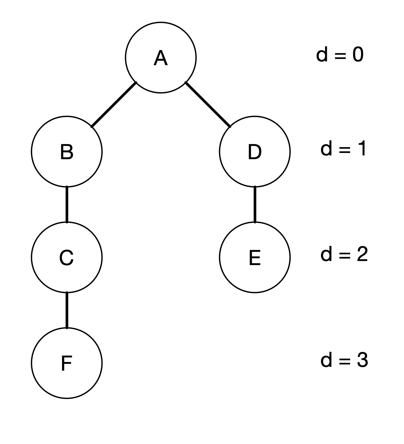
Notice that we can actually add F either to C or to E in the tree above. In this case, we choose to add to C. The question is when do we stop? We should stop when all the vertices have been explored in terms of their children. Therefore, we need some way to indicate if a Vertex's children have been fully explored. The way we are going to do this is to colour the vertices. Moreover, we are going to use three different colours:

• white: is used to indicate that we have not visited the vertex
• grey: is used to indicate that we have visited the vertex but we have not completely explored all the neighbours
• black: is when we have explored all the neighbours of this vertex.

With this in mind, the image below shows the progression of the vertex exploration and how the colour of each vertex changes.

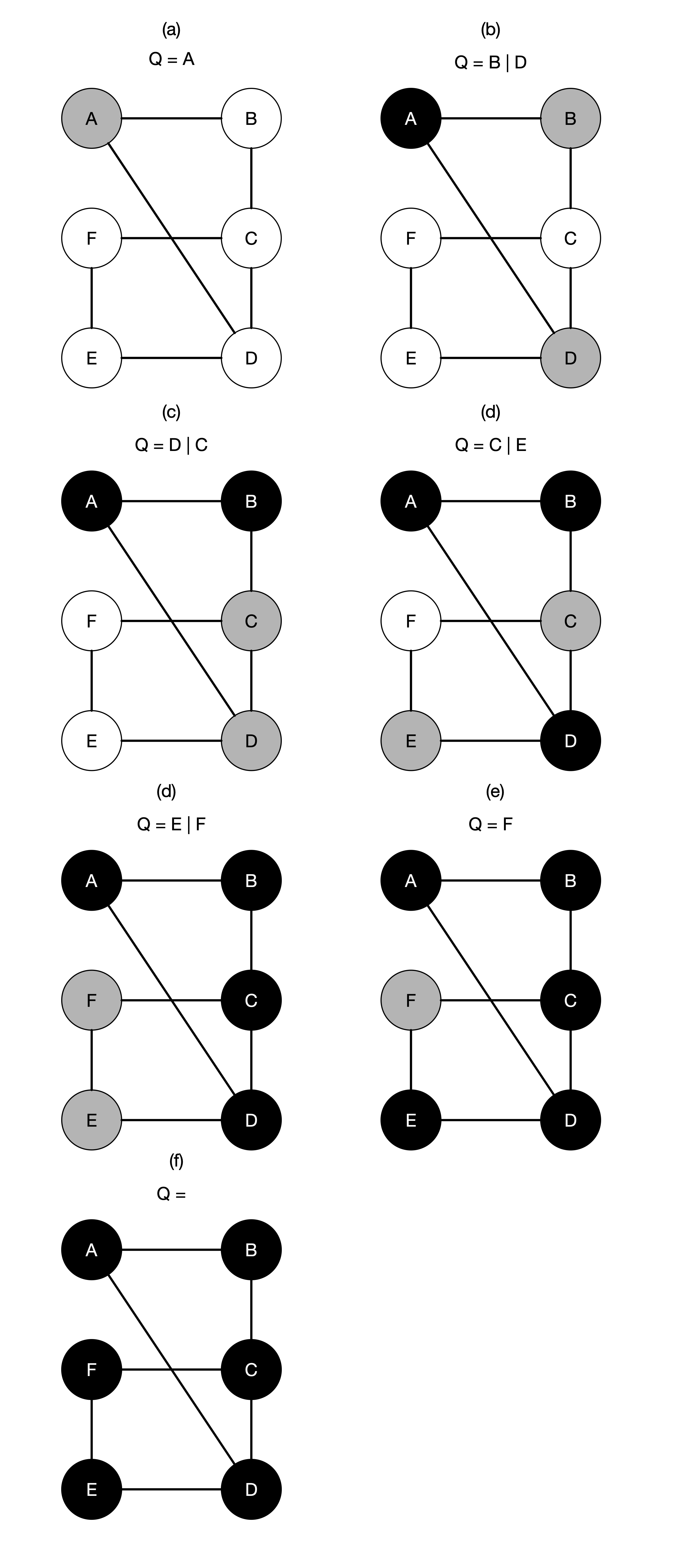
In the figures above, we use a Queue data structure to explore the vertices. When we visit vertex, we put all its neighbouring vertices into a queue. This also ensures that we explore the vertices in a breadth-first manner. For example, when we explore B from A, we did not go to C but rather D, which is at the same level as B in our search tree. This is where the name breadth-first search comes from. So now we are ready to write our algorithm for breadth-first search.

(D)esign of Algorithm

Show Pseudocode

Input:
- G: Graph
- s: starting vertex
Output:
- Graph with distances on every vertex from s
Steps:
1. Initialize every vertex with the following:
  1.1 set color to white
  1.2 set distance to INF
2. start from s vertex:
  2.1 set s' color to grey
  2.2 set s' distance to 0
3. put s into the Queue
4. As long as Queue is not empty
  4.1 take out one vertex from Queue and store to u
  4.2 for each neighbour of vertex u, do:
    4.2.1 if the neighbour colour is white, do:
      4.2.1.1 set the neighbour's colour to grey
      4.2.1.2 set the neighbour's distance to u's distance + 1
      4.2.1.3 put the neighbour into the Queue
  4.3 after finish exploring all neighbours, set u's color to black

In the above algorithm, we start by setting all the vertices to white and have a distance of INF (infinite) or any large number value greater than the number of the vertices. We then start from the vertex s and explore its neighbours. Everytime we explore a neighbour, we check its colour. If the colour is white, it means that it has not been visited previously, so we change the colour to grey and add the distance by one. We then put this neighbour into the queue to visit its neighbours later on. We proceed visiting the vertices by taking out the vertex from the Queue. As mentioned, it is the Queue that ensures that we visit the vertices in a breadth-first manner.

The only thing about this algorithm is that we only get a graph with distances on each vertex, but we would not be able to retrieve the path to take from s to the destination vertex. In order to find the shortest path, we need to store the parent vertex when we visit a neighbouring vertex. To do this, we modify the algorithm as follows.

Show Pseudocode

Input:
- G: Graph
- s: starting vertex
Output:
- Graph with:
  - distances on every vertex from s
  - parent vertex on every vertex that leads back to s
Steps:
1. Initialize every vertex with the following:
  1.1 set color to white
  1.2 set distance to INF
  1.3 set parent to NILL
2. start from s vertex:
  2.1 set s' color to grey
  2.2 set s' distance to 0
  2.3 set s' parent to NILL
3. put s into the Queue
4. As long as Queue is not empty
  4.1 take out one vertex from Queue and store to u
  4.2 for each neighbour of vertex u, do:
    4.2.1 if the neighbour colour is white, do:
      4.2.1.1 set the neighbour's colour to grey
      4.2.1.2 set the neighbour's distance to u's distance + 1
      4.2.1.3 set u as the parent vertex of the neighbour
      4.2.1.4 put the neighbour into the Queue
  4.3 after finish exploring all neighbours, set u's color to black

In the second algorithm, we have a new attribute called parent. In the beginning we set all vertices to have NILL as their parents. Since s is the starting vertex, it has no parent and so we set to NILL in step 2.3. We added step 4.2.1.3 where we set u as the parent to the neighbouring vertex when we add that neighbouring vertex into the Queue.

With this, we can write another algorithm to retrieve the path from s to some destination vertex v.

Show Pseudocode

Find-Path BFS
Input:
- G: graph after running BFS
- s: start vertex
- v: end vertex
Output:
- list of vertices that gives the shortest path from s to v
Steps:
1. if v is the same as the start vertex
  1.1 return a list with one element, i.e. s
2. otherwise, check if parent of v is NILL
  2.1 return "No path from s to v exist"
3. otherwise,
  3.1 call find-path(G, s, parent of v)
  3.2 add v into the result from 3.1

The above algorithm uses recursion. There are two base cases. The first base case is when the destination vertex to be the same as the starting vertex. In this case, the output is just that vertex. The second base case is when there is no path from s to v. We know there is no path when along the path starting from v we find a vertex which parent is NILL. The recursion case is described in step 3. In this case, we call the same function but with the destination vertex to be the parent of the current destination vertex. By moving the destination vertex to the parent, we reduce the problem and make it smaller until we reach base case described in step 1.

Let's see an example when we search a shortest path from A to F in the previous graph. In this case, v is not the same as s since A and F are two different vertices. So we look into F's parent, which is C. Now we call the same function to find the path from A to C. Since A and C are different, we look into C's parent, which is B and call the function to find the path from A to B. Finally, we look into B's parent and find the path from A to A. This is the base case. When we reach the base case, we return a list containing A as the result (step 1.1). Then we move back and do step 3.2 to add B, C, and finally F. So the shortest path from A to F will be a list [A, B, C, F].

Now it's time to implement the algorithm. But before we can implement the algorithm, we need to modify the class Vertex to contain a few additional attributes:

• colour
• distance
• parent

As mentioned in the Introduction, we will do this using the concept of Inheritance.

Inheritance

Inheritance is an important concept in object oriented programming that allows us to re-use existing code or classes we have written. In our example here, we already have a class Vertex and Graph. However, the class Vertex only contains id and neighbours.

As shown in the previous section, our Vertex object has additional attributes such as colour, distance, and parent. We can actually create a new class containing all these new properties as well as the commonly found properties of a vertex (id and neighbours). However, we will duplicate our codes and rewriting the methods that is the same for all Vertex objects such as adding a neighbour. Inheritance allows us to create a new class without duplicating all the other parts that is the same. By using inheritance, we create a new class by deriving it from an existing base class. In this example, we can create a new class called SearchVertex that is derived from a base class Vertex. When a class inherits another class, the new class possess all the attributes and methods of its parent class. This means that SearchVertex class contains both id and neighbours as well as all the methods that Vertex class has. What we need to do is simply to specify what is different with SearchVertex that Vertex class does not have. We can represent this relationship using a UML diagram as shown below.

In the UML diagram, the relationship is represented as an arrow with a white triangle pointing from the child class to the parent class. This relationship is also called is-a relationship which simply means that SearchVertex is-a Vertex, it has all the attributes and methods of a Vertex object.

In Python, we can specify if a class derives from another class using the following syntax:

class NameSubClass(NameBaseClass):
    pass

For our example here, we can write the SearchVertex class as follows.

class SearchVertex(Vertex):
    pass

In the above class definition, we have Vertex inside the parenthesis to indicate to Python that we will use this as the parent class or base of SearchVertex class. In this new class, we can initialize all the new attributes as usual:

import sys

class SearchVertex(Vertex):
    def __init__(self, id=""):
        super().__init__(id)
        self.colour = "white"
        self.d = sys.maxsize
        self.parent = None

Notice here that we initialize:

• colour to be "white"
• d to be a large integer number
• parent to be a None object

The first line super().__init__(id) is to call the parent class' initialization method to initialize the both the id and the neighbours. The word super comes from Latin which means "above". Therefore, super() method returns a reference to the parent's class. Since we have both __init__() method in SearchVertex and Vertex, we need to be able to differentiate the two methods. For this purpose, Python provides super() method to refer to the parent's class methods instead of the current class.

In the child class SearchVertex we redefine the __init__() method of the parent's class. This is what is called as method overriding.

tip

Try it out in the interactive code editor below

The first line of the init is to call the parent class' initialization and the subsequent lines proceed to initialize those attributes that is unique to the child class. In this way, we need not re-write all the initialization codes of the parent class and simply re-use them. Note that in overriding a method in the parent class, we use the same method's name and arguments as in the parent class.