Depth First Search
Depth-first search (DFS) is a crucial graph traversal algorithm that explores as far as possible along each branch before backtracking. This depth-wise exploration makes DFS particularly effective for tasks such as topological sorting, cycle detection, and solving puzzles. Topological sorting is used to order tasks based on dependencies, ensuring that prerequisite tasks are completed first. For example, in project management software, DFS can help determine the sequence of tasks to optimize workflow. Cycle detection is another important application, where DFS identifies cycles in graphs, which is essential for detecting deadlocks in operating systems or circular dependencies in software packages. Additionally, DFS is employed in solving puzzles with a unique solution, such as mazes or Sudoku. By systematically exploring all possible paths, DFS can find the correct sequence of moves to solve the puzzle.
Depth-first search (DFS) is a versatile algorithm with numerous applications in Artificial Intelligence (AI). Here are some examples of how DFS is used in AI:
-
Pathfinding in Games:
- DFS is used to explore possible moves in games like chess or checkers. By traversing the game tree deeply, AI can evaluate potential strategies and determine the best move to make.
-
Web Crawling:
- Search engines use DFS to crawl web pages. Starting from a given URL, DFS explores links deeply to index content, ensuring comprehensive coverage of the web.
-
Solving Constraint Satisfaction Problems:
- In problems like Sudoku or the N-Queens puzzle, DFS systematically explores possible configurations to find solutions that satisfy all constraints.
-
Automated Planning:
- In AI planning, DFS helps in exploring possible sequences of actions to achieve a goal. This is particularly useful in robotics and automated systems where the algorithm can find optimal paths for task execution.
-
Genetic Algorithms:
- DFS can be employed to explore the search space in genetic algorithms, helping to identify optimal solutions by deeply traversing possible genetic variations.
These examples illustrate the broad applicability of DFS in AI, from game strategy and web indexing to solving complex puzzles and optimizing neural networks. The depth-wise exploration characteristic of DFS makes it a powerful tool for efficiently tackling a wide range of AI problems.
Goals
By the end of this lesson, you should be able to:
- explain and implement depth first search.
depth first search, topological search, colour, parent vertex, start/finish time
Depth-First Search
There is another kind of search that can be done on a graph. This is called depth-first search (DFS). As the name implies, this algorithm explores the neighbouring vertices in a depth-wise manner. DFS is used in topological sorting, scheduling problems, cycle detection in graph and solving puzzles with only one solution such as finding a path in a maze or solving a sudoku puzzle. Let's illustrate this with the same graph as we have seen previously.
(C)ases
We will now give an example of a depth first search algorithm. Recall that breadth first search creates a BFS tree. On the other hand, depth first search algorithm creates a forest. A forest is a collection of trees (and yes, it can consist of a single tree). More formally, a forest is a disjoint union of trees. Let's see how the algorithm works. In the below example, our forest consists only of a single tree.
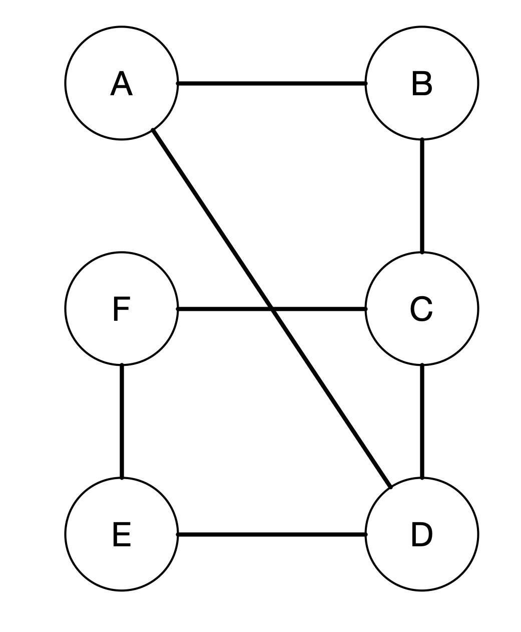
In depth-first search, we go down the tree before moving to the next siblings. For example, as we start from A, we look into its neighbouring vertices. So vertex A has two neighbours, i.e. B and D. The depth-first search algorithm will visit one of them, say vertex B. After it visits B, it will explore one of the neighbours of B instead of visiting D. This is illustrated below.

In the figures above, every time we visit a vertex, we put a timestamp on that vertex called discovery time. Once we finish visiting all the neighbours of that vertex, we put another timestamp called finishing time. For example, vertex A has a discovery time 1 and finishing time 12 as indicated by 1/12 in the figure.
We also labelled the edges with two different kind of symbols. The solid line edges are called tree edges. These are edges in the depth-first forest. An edge (u, v) is a tree edge if v was first discovered by exploring edge (u, v). For example, the edge (A, B) is a tree edge since B is first discovered by exploring the edge (A, B). On the other hand the edge (A, D) is not a tree edge since D was not first discovered by exploring edge (A, D). Rather, D was first discovered by exploring the edge (C, D).
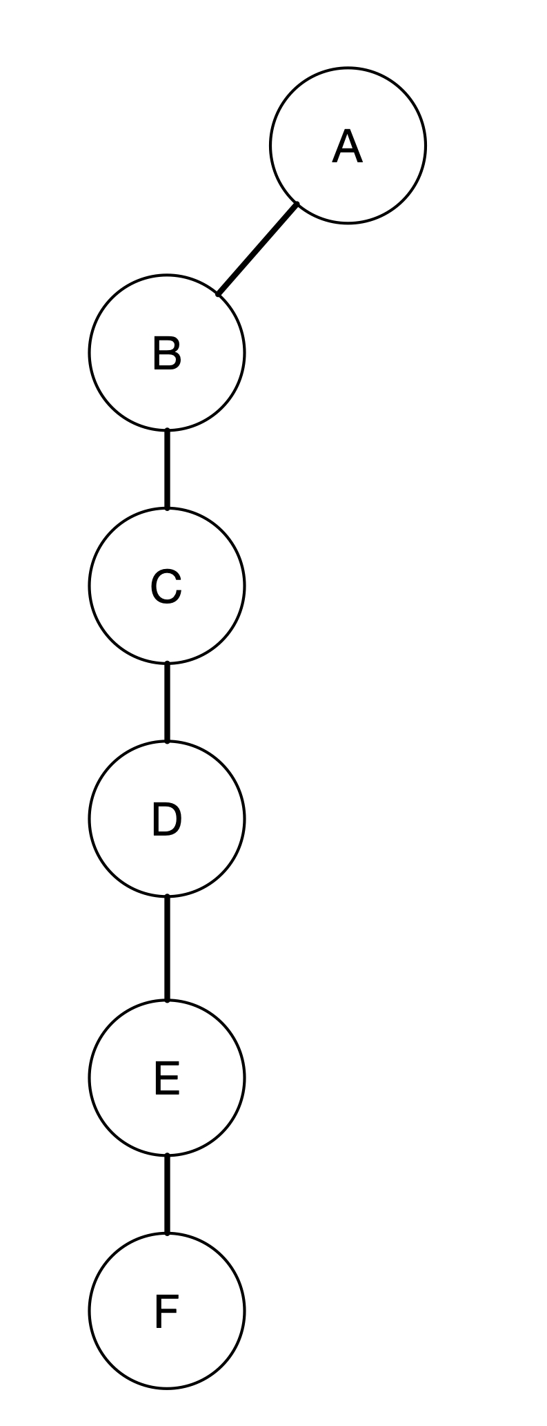
This brings us to the other kind of edges discovered by depth-first search. The dashed line edges are called back edges. These are those edges connected a vertex u to an ancestor v in a depth-first tree. For example, A is an ancestor of D. We can see that because we explore D through A - B - C - D. So the edge connecting D to A is a back edge since it connects D to one of its ancestor. Similarly with the edge (C, F). The depth-first forest is shown below.
(D)esign of Algorithm
Now we can try to write the steps to do depth-first search. We will write the steps using two functions. The first one is called DFS as shown below.
Show Pseudocode
DFS
Input:
- G: graph
Output:
- G: graph with the following attributes marked
  - colour
  - discovery time
  - finishing time
  - parent
Steps:
1. Initialize each vertex as follows:
  1.1 set colour to white
  1.2 set parent to NILL
2. set time to 0
3. for each vertex in the graph G
  3.1 if the vertex's colour is white, do:
    3.1.1 dfs-visit(G, u)
The above algorithm simply initialize the vertices and go through every vertex to perform the second function DFS-VISIT.
Show Pseudocode
DFS-Visit
Input:
- G: graph
- u: vertex to visit
Output:
- G: graph with the following attributes marked
  - colour
  - discovery time
  - finishing time
  - parent
Steps:
1. increase time by 1
2. set current time to be the discovery time for u
3. set u's colour to gray
4. for each vertex in u's neighbours, do:
  4.1 if the vertex's colour is white, do:
    4.1.1 set u as the parent of the vertex
    4.1.2 call dfs-visit(G, the current vertex)
5. set u's colour to black
6. increase time by 1
7. set current time to be the finishing time
This function simply set the discovery time for the visited vertex u and begins to visit all the neighbouring vertices of u. However, it only calls DFS-VISIT if the neighbouring vertices are white, which means these vertices have not been visited yet. Once it finishes visiting all the neighbouring vertices, it marks the vertex u to be black and set the finishing time.
Topological Sort
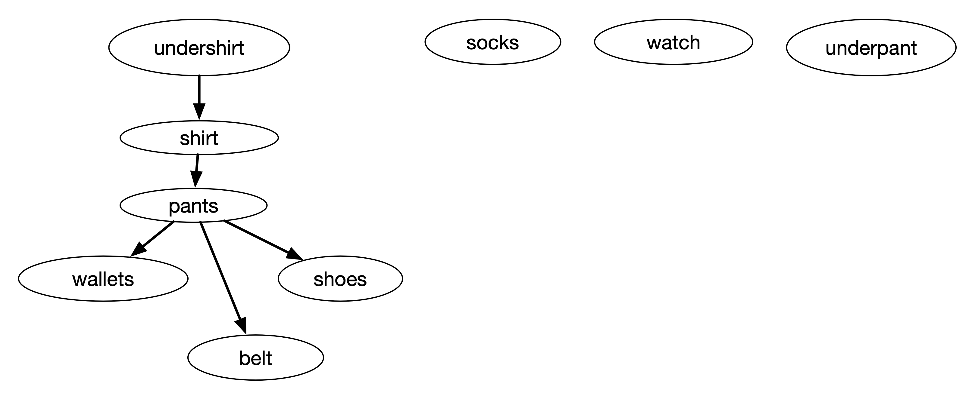
One application of depth-first search algorithm is to perform a topological sort. For example, if we have list of task with dependencies, we can sort which task should be performed first. The figure below gives an example of this dependencies tasks
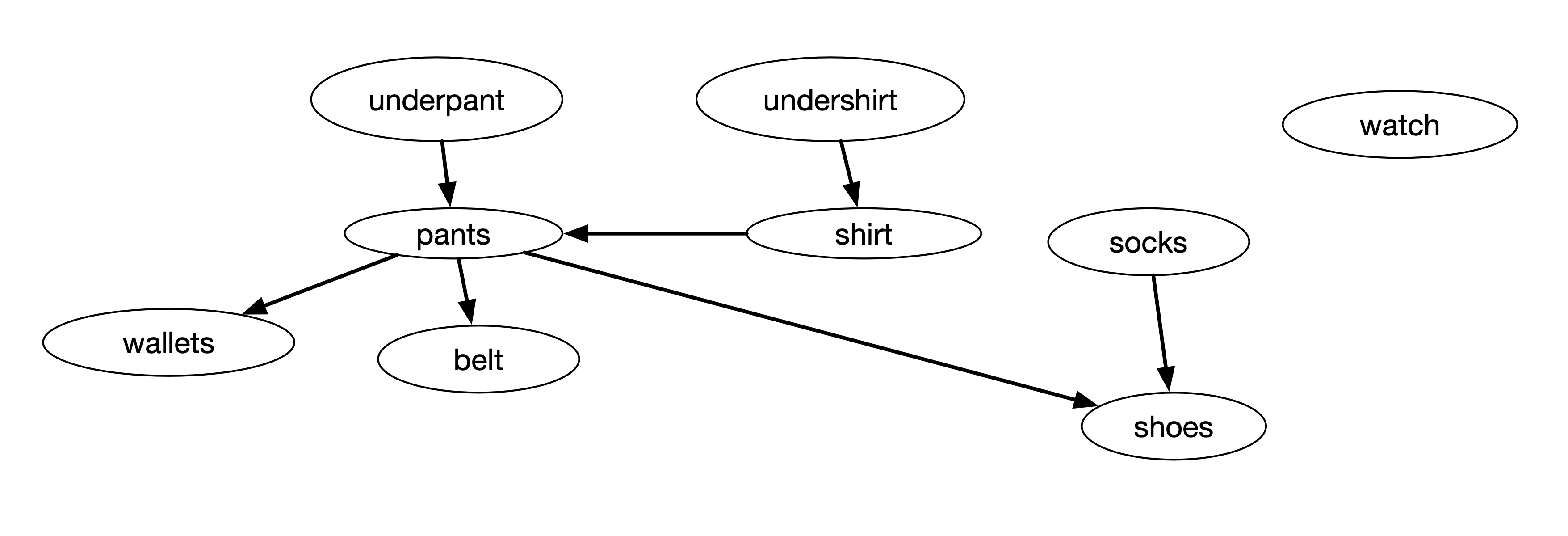
The figure above shows a directed graph of dependencies between different tasks. For example, the task wearing a pant must be done only after the task of wearing underpant and wearing a shirt. We can use the finishing time of DFS to determine the sequence of tasks.
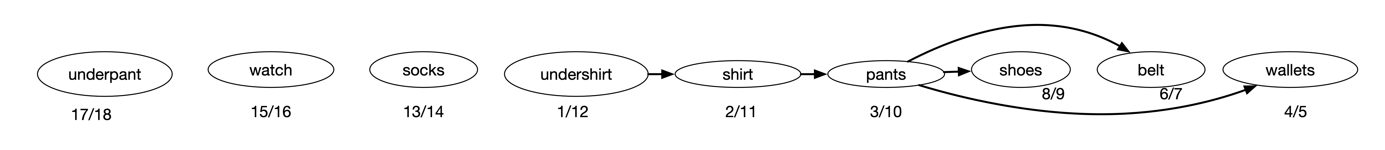
Let's try to perform DFS for the above graph. The discovery time and the finishing time for each task is shown in the figure below.
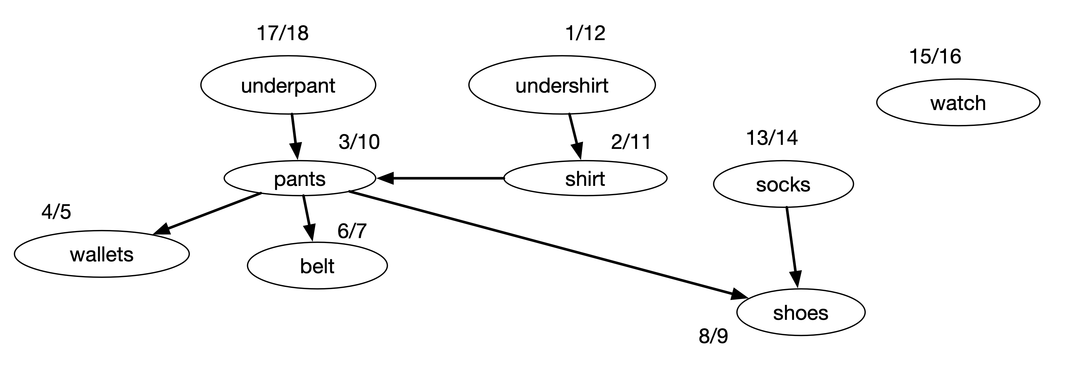
In the process of DFS, it starts with "undershirt" and traverse to all the children vertices in the tree, i.e. "pants", "wallets", "belt", and then "shoes". After this, it creates another tree starting from "socks", and then another tree starting from "watch", and finally another tree starting from "underpant". The DFS can actually starts from "socks" or "watch" or "underpant". But each of these will have no other vertex to go to and remain as a single vertex. Our DFS algorithm can be modified to specify which vertex to start from or it can be determined based on the goal. Currently, it starts aribitrarily and it picks "undershirt" first.
The depth-first forest looks like the figure below.
We can re-order the tasks by its finishing time from the largest to the smallest as shown in the figure below.
The sequence above is based on its finishing time from the largest to the smallest. The first three are independent and their sequence can be interchanged, but subsequently, "shirt" must be done only after "undershirt" task. This sequence may also depends on which vertex the search encounters first. With this in mind, we can write the topological sort steps as follows.
Show Pseudocode
Topological-Sort
Input:
- G: graph
Output:
- list of sorted vertices
Steps:
1. call DFS(G) to compute the finishing time for each vertex in G
2. sort the vertices based on its finishing time from largest to smallest
3. return a list of sorted vertices